How to build a license plate recognition system
As I'm learning about computer vision, I built a prototype of a license plate recognition system to get familiar with some of the tools and concepts used the field. This is a summary of how I built such as a system and how it works.
What I mean by license plate recognition
Automatic Number Plate Recognition (ANPR) systems take a video feed or a static image and extract the license plate number of any vehicles shown. They are widely used for vehicle recognition, access control, parking-spot management, etc. In general, an ANPR system consists of two elements, a sub-system that identifies the license plate in the image or video, and another one that extracts and interprets the alphanumeric characters. This project is only concerned with the first part, the identification of license plates in car images.
Furthermore, ANPR systems can be classified in two groups:
-
Fixed systems, which are installed at a given location and do not move (hence the name). These are the systems that are used, among other things, to identify vehicles at a parking entrance. When working with fixed systems, the car images are all taken, more or less, from the same distance and at the same angle.
-
Mobile systems, which are portable and designed to be used in a wider range of circumstances. They are used, for example, by law enforcement to identify vehicles.
Here, I am modelling a fixed ANPR system, thus, in all data images, the relative position between the camera and the car is more or less the same.
I used data from the Department of Electronics, Microelectronics, Computer and Intelligent Systems of the Faculty of Electrical Engineering and Computing of the University of Zagreb to develop and test the system, but the techniques and implementation should work on any dataset with minor adjustments.
Design overview
When given an image of the rear part of a car, the license plate recognition system should be able to choose which part of the image corresponds to the license plate. In order to simplify this task, I considered the hypothetical ANPR system to be fixed, i.e., the relative pose (distance and orientation) of the cars with respect to the camera is somewhat constant across different images. Based on this, it can be assumed that the license plate in all images is going to be around the same size. Thus, if the license plate size is known, the system just needs to be able to tell which of all the possible sub-images of that size looks more like a license plate.
All images in the dataset I used are 640 pixels by 480, and by inspecting them, it's easy to see that the size of the license plate in most cases is about 300 pixels by 64. I should point out that some of the images in the database show special vehicles, such as heavy trucks, which have plates of different shapes or colors. To keep thing simple, I didn't consider those special plates for this first prototype.
The license plate recognition algorithm is then designed to work in the following manner:
-
It takes an image of size 640x480.
-
It crops the image to generate some number of sub-images of size 300x64. The cropping should be done in a way that ensures that one of these sub-images shows the entire license plate.
-
It applies a classification algorithm to identify which of the sub-images contains the license plate.
The classification algorithm
To distinguish between the 300x64 images that show a license plates and the ones that don't, I used a classification algorithm based on the k-nearest-neighbors (knn) method. In general, this algorithm works by taking some piece of data and assigning it to one of a set of categories, which are known in advanced. This is achieved by first exposing the algorithm to a training dataset, composed of data points of which the category to which they belong is known. When a new data point is given to the algorithm, it compares it to the points in the training data set to find one that resemble the new data point. The training data points that are similar to the new one are called its nearest-neighbors. The new data point is assigned to the same category as its nearest-neighbors.
The way this is technically implemented requires a way of describing the data points using numerical properties. For example, let's say that we want to classify animals into the categories "cat" and "sheep". We can describe animals using their weight and height, thus we'll need a training dataset which will consist of the weight and height of some sheep and some cats. When the system is presented with a new animal, it compares the weight and height of the mysterious creature with the training data set. If both values are relatively similar to the values corresponding to the cats in the training dataset, then it's a cat, if it's closer to a sheep, then it's a sheep.
Mathematically, the numerical properties used to describe the data points can be used to construct a vector space. Since in this example we only have two properties, weight and height, the space will be two-dimensional and we can represent the training data-points as literal points:

When the algorithm is given a new point that needs to be classified, a new animal of unknown specie, its weight and height can be represented on the same plot:

Intuitively, it's easy to see that the new animal is more likely to be a cat than a sheep. Mathematically, the closest training point is of type "cat", so the new point is also assigned to the same category. It should be noted that we can check more than one of the nearest neighbors; both the number of nearest-neighbors that are considered and the mathematical definition of "nearest" can be tweaked when applying the algorithm.
The histogram of oriented gradients
I used the k-nearest-neighbors algorithm classify the sub-images into the categories "license plate" or "other", but in order to apply it, I needed a way of describing the images using a set of numerical values, like the weight and height in the example. The histogram of oriented gradients (HOG) is a method used to describe images using numerical values that was popularized in a 2005 paper by N. Dalal and B. Triggs that used it to identify pedestrian in images. It works as follows:
-
First, the gradients of all the pixels in the image are calculated. The gradient is a mathematical concept that measures how much a multi-variable function changes. In the case of an image, it gives an idea of how different a given pixel is from the ones in its surroundings. In particular, the gradient is composed of two things, the direction in which the most different pixel can be located, and a measurement of how different that other pixel is. The HOG descriptors are built using the former.
-
Once the first step is completed, I have, for each pixel, a value that indicates the direction of maximum change. These directions can be expressed as an angle, for example, if the most different pixel is completely to the right, that can be 0°, if it's straight up, then it would be 90°, and so on. In order to simplify the data, the angle values are then grouped together in buckets of amplitude 20°, i.e., any angle from 0° to 20°, goes to the first bucket, any angle from 20° to 40° to the second one, and so on.
-
Nearby pixels are grouped into cells. The cells are non-overlapping and their size can be specified as an algorithm-parameter.
-
At this point, we have divided the images into cells. Each cell has a given number of pixels and each pixel has a gradient-angle associated with it. Also, the gradient-angles are grouped into a small number of buckets. The next step is to build, for each cell, a histogram that describe how the angles of the pixels in that cells are distributed among the different buckets.
-
Finally, we group the cells into blocks. The different between a cell and a block is that blocks are overlapping, this is, a single cell can belong to multiple blocks. The HOG descriptor of the image is then a vector that contains the normalized angle-histograms of every block.
If you want to know more about the HOG algorithm, but don't want to read the academic paper, here you can find a more detailed explanation with nice graphics and animations.
The takeaway is that the HOG method can be used to obtain numerical descriptors of images that can then be fed into the k-nearest-neighbors classification algorithm.
Implementation
I implemented the prototype in Matlab, using the Computer Vision Toolbox, the Image Processing Toolbox, and the Statistics and Machine Learning Toolbox. The complete implementation can be found on my Github.
Training data
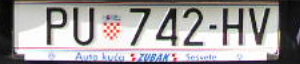
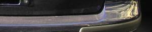
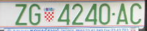
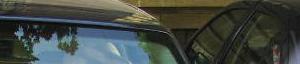
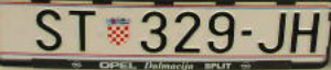
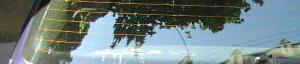
The images I used to train the algorithm can be found here. For each of the training images, I manually selected a 300x64 sub-image that matched the license plate of the vehicle, to be used as a training data point for the "license plate" category. For the "other" training data, I cropped each of the training images into random sub-images of size 300x64. Then, I manually revised these sub-images to remove any that contain parts of the license plates. Here are some examples of the images used for training, both for the "license plate" and "other" categories:
The HOG descriptors of the training images are computed using the
extractHOGFeatures()
function from the Computer Vision Toolbox and saved in a binary data file so that they
can be used latter on:
train_plate_dir = "data/training/plates";
train_no_plate_dir = "data/training/non_plates";
save_data_dir = "data/training";

train_plate_filenames = dir(fullfile(train_plate_dir, "*.png"));
train_no_plate_filenames = dir(fullfile(train_no_plate_dir, "*.jpg"));
all_plates_hf = [];

% Hog values from plate images
for i=1:length(train_plate_filenames)
    full_name = fullfile(train_plate_dir, train_plate_filenames(i).name);
    image = imread(full_name);
    hf = extractHOGFeatures(image);
    all_plates_hf(i, :) = hf;

end

all_no_plates_hf = [];
% Hog values from non-plate images
for i=1:length(train_no_plate_filenames)
    full_name = fullfile(train_no_plate_dir, train_no_plate_filenames(i).name);
    image = imread(full_name);
    hf = extractHOGFeatures(image);
    all_no_plates_hf(i, :) = hf;

end

save(fullfile(save_data_dir, "hog_features"), "all_no_plates_hf", "all_plates_hf");
The complete system
I used the fitcknn() function from
the Statistics and Machine Learning Toolbox to build a knn classifier using training
data-points:
load("data/training/hog_features");

[n_plates, ~] = size(all_plates_hf);
[n_other, ~] = size(all_no_plates_hf);
all_training_data = [all_plates_hf; all_no_plates_hf];
labels = [
    repmat("plate", n_plates, 1);
    repmat("other", n_other, 1)
    ];

model = fitcknn(all_training_data, labels);
Then, I tested the classifier to be sure that it could differentiate between the sub-images that show a license plate and the ones that don't:
test_dir = "data/test_classifier/";
should_be_plate = ["P6070066_plate.jpg", "P6070075_plate.jpg"];
should_not_be_plate = [
    "P6070066_non_plate_1.jpg" ...
    "P6070066_non_plate_2.jpg" ...
    "P6070066_non_plate_3.jpg" ...
    "P6070075_non_plate_1.jpg" ...
    "P6070075_non_plate_2.jpg" ...
    "P6070075_non_plate_3.jpg" ...
    ];
all_test_filenames = [should_be_plate, should_not_be_plate];
complete_test_dataset = [];
expected_test_results = [];

% Test images that are license plates
for i=1:length(should_be_plate)
    filepath = fullfile(test_dir, should_be_plate(i));
    img = imread(filepath);
    hf = extractHOGFeatures(img);
    complete_test_dataset = [complete_test_dataset; hf];
    expected_test_results = [expected_test_results; "plate"];
end
save("data/classifier", "model")

% Test images that are not license plates
for i=1:length(should_not_be_plate)
    filepath = fullfile(test_dir, should_not_be_plate(i));
    img = imread(filepath);
    hf = extractHOGFeatures(img);
    complete_test_dataset = [complete_test_dataset; hf];
    expected_test_results = [expected_test_results; "other"];
end

test_results = model.predict(complete_test_dataset);
for i=1:length(test_results)
    if test_results{i} == expected_test_results(i)
        disp("Test passed: " + all_test_filenames(i))
    else
        disp("Test: failed" + all_test_filenames(i))
    end
end
For the tests, I used images that were not in the training set, and the classifier passed all all of them.
Finally, I put all the parts together; the complete system takes an input image, divides it into sub-images using constant horizontal and vertical intervals, and computes the HOG descriptors of all the sub-images. Then, it uses the knn classifier to select the sub-image(s) that best qualify as license plates. In the case that two or more sub-images are tied as the best ones, the method averages their x-y coordinates, since it's probably caused by multiple images containing different sections of the license plate:
rows_step = 5;
cols_step = 10;
section_width = 300;
section_heigth = 64;

n_rows = 480;
n_cols = 640;

image_filename = fullfile(images_dir, test_filename);
image = imread(image_filename);
upper_left_corner = [1,1];

max_row = n_rows - section_heigth;
max_cols = n_cols - section_width;
left_upper_corner = [];
predictor_data = [];
for i=1:rows_step:max_row
    for j=1:cols_step:max_cols
        left_upper_corner = [left_upper_corner; [j, i]];
        disp("row: " + num2str(i) + ", column: " + num2str(j))
        sub_image = imcrop(image, [j, i, section_width, section_heigth]);
        hf = extractHOGFeatures(sub_image);
        predictor_data = [predictor_data; hf];
    end
end
[label, score, cost] = model.predict(predictor_data);
score_plate = score(:, 2);
best_scores_idx = find(score_plate == max(score_plate));

x_rectangle_values = zeros(1, length(best_scores_idx));
y_rectangle_values = zeros(1, length(best_scores_idx));
for i=1:length(best_scores_idx)
    idx = best_scores_idx(i);
    x_rectangle_values(i) = left_upper_corner(idx, 1);
    y_rectangle_values(i) = left_upper_corner(idx, 2);
end

rectangle_position = [floor(mean(x_rectangle_values)), floor(mean(y_rectangle_values))];
As it can be here the results are quite nice for such a simple prototype:
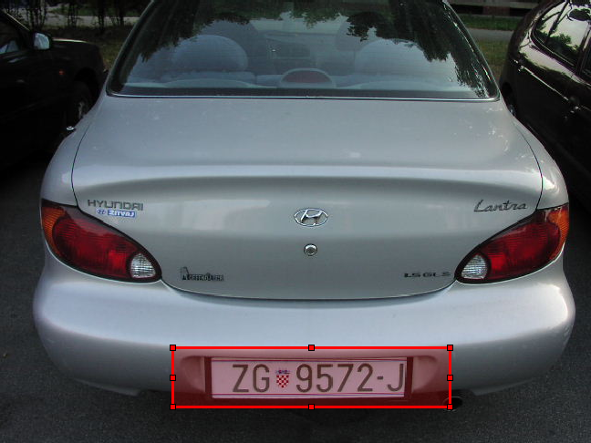
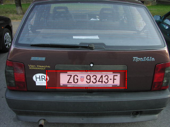
One problem with the system seems to be that the dimensions of the license plate across different images is not as constant as I was expecting. As a result, in some images, even though the algorithm selects the correct area, the 300x64 selection is too large.
Another thing I'd like to have a look at is the method used to generate the sub-images from the complete image. Here, I used the simplest approach, cropping the image at constant intervals, but it would be nice to investigate more efficient ways of doing it.
All in all, I'm quite happy with the system, the results are better that what I was expecting, and it was nice to apply these techniques to a small project such as this one.